Analysis of solvation shells

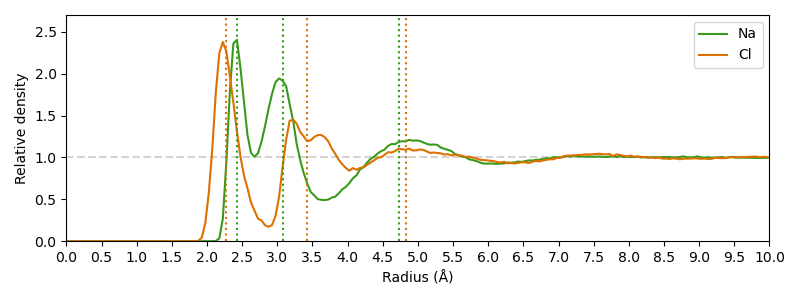
Based on a 10 ns Gromacs MD simulation of 0.15 mM sodium chloride, the distance of solvation shells to the central ion for both, sodium and chloride ions, are analyzed.

For this purpose the radial distribution function (RDF) is calculated for water molecules (specifically the oxygen atom) centered on these ions.

The trajectory file can be downloaded here and the template PDB can be downloaded here.

Two things are peculiar in this plot: At first, the first solvation shell has a smaller distance from chloride ions than from sodium ions, although the radius of chlorine is higher. Furthermore, the second solvation shell of the chloride ions seems to be separated into two distinct peaks.

# Code source: Patrick Kunzmann
# License: BSD 3 clause

import matplotlib.pyplot as plt
import numpy as np
import scipy.signal as signal
import biotite
import biotite.structure as struc
import biotite.structure.io as strucio

# Put here the path of the downloaded files
templ_file_path = "../../../download/waterbox_md.pdb"
traj_file_path = "../../../download/waterbox_md.xtc"

# Load the trajectory
traj = strucio.load_structure(traj_file_path, template=templ_file_path)
# Sanitize the PDB file produced by Gromacs:
# Use capital letters for atom elements...
traj.element = np.array([element.upper() for element in traj.element])
# ...and set 'hetero' to true for all atoms,
# as the file does not contain any regular chains.
traj.hetero[:] = True

# Create boolean masks for all sodium or chloride ions, respectively
na = traj.coord[:, traj.element == "NA"]
cl = traj.coord[:, traj.element == "CL"]
# Create a boolean mask for all watewr molecules
solvent = traj[:, struc.filter_solvent(traj)]
# Calculate the RDF of water molecules
# centered on sodium or chloride ions, respectively
N_BINS = 200
bins, rdf_na = struc.rdf(center=na, atoms=solvent, periodic=True, bins=N_BINS)
bins, rdf_cl = struc.rdf(center=cl, atoms=solvent, periodic=True, bins=N_BINS)

# Find peaks
# This requires a bit trial and error on the parameters
# The 'x' in '[x * N_BINS/10]' is the expected peak width in Å,
# that is transformed into a peak width in amount of values
peak_indices_na = signal.find_peaks_cwt(rdf_na, widths=[0.2 * N_BINS / 10])
peak_indices_cl = signal.find_peaks_cwt(rdf_cl, widths=[0.3 * N_BINS / 10])
peak_indices_na, peak_indices_cl = peak_indices_na[:3], peak_indices_cl[:3]

# Create plots
fig, ax = plt.subplots(figsize=(8.0, 3.0))
# Plot average density in box
ax.axhline(1, color="lightgray", linestyle="--")
# Plot both RDFs
ax.plot(bins, rdf_na, color=biotite.colors["darkgreen"], label="Na")
ax.plot(bins, rdf_cl, color=biotite.colors["dimorange"], label="Cl")
# The peak positions are shown as vertical lines
ax.vlines(
    bins[peak_indices_na],
    ymin=0,
    ymax=3,
    color=biotite.colors["darkgreen"],
    linestyle=":",
)
ax.vlines(
    bins[peak_indices_cl],
    ymin=0,
    ymax=3,
    color=biotite.colors["dimorange"],
    linestyle=":",
)
ax.set_xticks(np.arange(0, 10.5, 0.5))
ax.set_xlim(0, 10)
ax.set_ylim(0, 2.7)
ax.set_xlabel("Radius (Å)")
ax.set_ylabel("Relative density")
ax.legend()

fig.tight_layout()
plt.show()