Note
Go to the end to download the full example code
Hydropathy and conservation of ion channels#
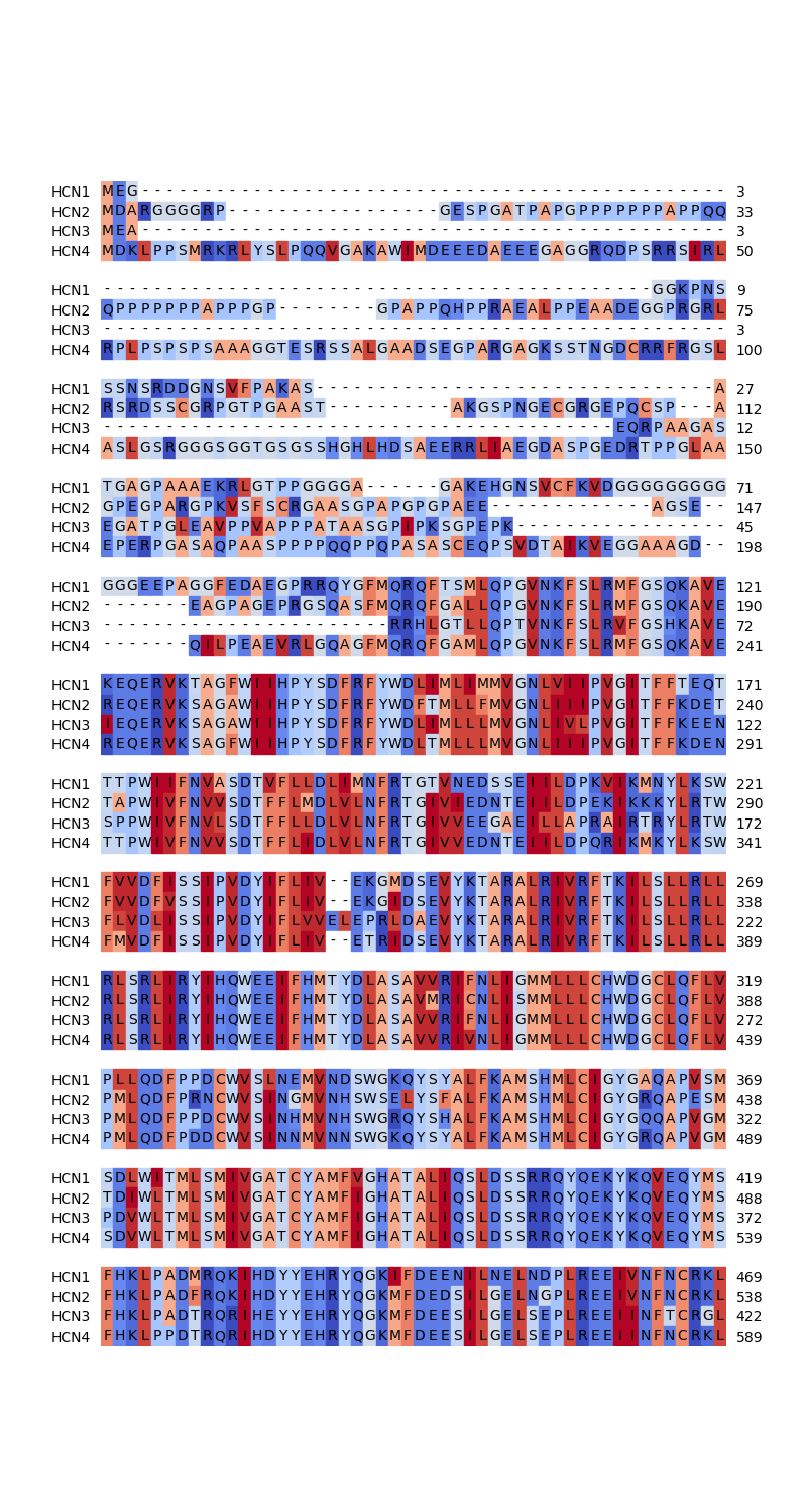
This script creates a hydropathy plot of the human HCN1 channel protein and compares it with the positional conservation within the HCN family. Eventually, an alignment of the HCN family is visualized using colors highlighting the hydropathy of the amino acid.
The HCN1 sequence is required for the hydropathy calculation. As the sequence annotation is also needed for the comparison of the hydropathy with the actual position of the transmembrane helices, the corresponding GenPept file is downloaded.
# Code source: Patrick Kunzmann
# License: BSD 3 clause

import matplotlib.pyplot as plt
import numpy as np
from matplotlib.patches import Patch
import biotite
import biotite.application.mafft as mafft
import biotite.database.entrez as entrez
import biotite.sequence as seq
import biotite.sequence.align as align
import biotite.sequence.graphics as graphics
import biotite.sequence.io.fasta as fasta
import biotite.sequence.io.genbank as gb

# Taken from
# Kyte, J and Doolittle, RF.
# "A simple method for displaying
# the hydropathic character of a protein".
# Journal of Molecular Biology (2015). 157(1):105–32.
# doi:10.1016/0022-2836(82)90515-0
hydropathy_dict = {
    "I": 4.5,
    "V": 4.2,
    "L": 3.8,
    "F": 2.8,
    "C": 2.5,
    "M": 1.9,
    "A": 1.8,
    "G": -0.4,
    "T": -0.7,
    "S": -0.8,
    "W": -0.9,
    "Y": -1.3,
    "P": -1.6,
    "H": -3.2,
    "E": -3.5,
    "Q": -3.5,
    "D": -3.5,
    "N": -3.5,
    "K": -3.9,
    "R": -4.5,
}

# Look for the Swiss-Prot entry contaning the human HCN1 channel
query = (
    entrez.SimpleQuery("HCN1", "Gene Name")
    & entrez.SimpleQuery("homo sapiens", "Organism")
    & entrez.SimpleQuery("srcdb_swiss-prot", "Properties")
)
uids = entrez.search(query, db_name="protein")

gp_file = gb.GenBankFile.read(
    entrez.fetch(uids[0], None, "gp", db_name="protein", ret_type="gp")
)
hcn1 = seq.ProteinSequence(gb.get_sequence(gp_file, format="gp"))
print(hcn1)
MEGGGKPNSSSNSRDDGNSVFPAKASATGAGPAAAEKRLGTPPGGGGAGAKEHGNSVCFKVDGGGGGGGGGGGGEEPAGGFEDAEGPRRQYGFMQRQFTSMLQPGVNKFSLRMFGSQKAVEKEQERVKTAGFWIIHPYSDFRFYWDLIMLIMMVGNLVIIPVGITFFTEQTTTPWIIFNVASDTVFLLDLIMNFRTGTVNEDSSEIILDPKVIKMNYLKSWFVVDFISSIPVDYIFLIVEKGMDSEVYKTARALRIVRFTKILSLLRLLRLSRLIRYIHQWEEIFHMTYDLASAVVRIFNLIGMMLLLCHWDGCLQFLVPLLQDFPPDCWVSLNEMVNDSWGKQYSYALFKAMSHMLCIGYGAQAPVSMSDLWITMLSMIVGATCYAMFVGHATALIQSLDSSRRQYQEKYKQVEQYMSFHKLPADMRQKIHDYYEHRYQGKIFDEENILNELNDPLREEIVNFNCRKLVATMPLFANADPNFVTAMLSKLRFEVFQPGDYIIREGAVGKKMYFIQHGVAGVITKSSKEMKLTDGSYFGEICLLTKGRRTASVRADTYCRLYSLSVDNFNEVLEEYPMMRRAFETVAIDRLDRIGKKNSILLQKFQKDLNTGVFNNQENEILKQIVKHDREMVQAIAPINYPQMTTLNSTSSTTTPTSRMRTQSPPVYTATSLSHSNLHSPSPSTQTPQPSAILSPCSYTTAVCSPPVQSPLAARTFHYASPTASQLSLMQQQPQQQVQQSQPPQTQPQQPSPQPQTPGSSTPKNEVHKSTQALHNTNLTREVRPLSASQPSLPHEVSTLISRPHPTVGESLASIPQPVTAVPGTGLQAGGRSTVPQRVTLFRQMSSGAIPPNRGVPPAPPPPAAALPRESSSVLNTDPDAEKPRFASNL
The positional hydropathy is calculated and smoothened using a moving average for clearer visualization.
hydropathies = np.array([hydropathy_dict[symbol] for symbol in hcn1])


def moving_average(data_set, window_size):
    weights = np.full(window_size, 1 / window_size)
    return np.convolve(data_set, weights, mode="valid")


# Apply moving average over 15 amino acids for clearer visualization
ma_radius = 7
hydropathies = moving_average(hydropathies, 2 * ma_radius + 1)
In order to assess the positional conservation, the sequences of all human HCN proteins are downloaded and aligned.
names = ["HCN1", "HCN2", "HCN3", "HCN4"]

uids = []
for name in names:
    query = (
        entrez.SimpleQuery(name, "Gene Name")
        & entrez.SimpleQuery("homo sapiens", "Organism")
        & entrez.SimpleQuery("srcdb_swiss-prot", "Properties")
    )
    uids += entrez.search(query, db_name="protein")

fasta_file = fasta.FastaFile.read(
    entrez.fetch_single_file(uids, None, db_name="protein", ret_type="fasta")
)

for header in fasta_file:
    print(header)

sequences = []
for seq_str in fasta_file.values():
    sequences.append(seq.ProteinSequence(seq_str))

alignment = mafft.MafftApp.align(sequences)
sp|O60741.3|HCN1_HUMAN RecName: Full=Potassium/sodium hyperpolarization-activated cyclic nucleotide-gated channel 1; AltName: Full=Brain cyclic nucleotide-gated channel 1; Short=BCNG-1
sp|Q9UL51.3|HCN2_HUMAN RecName: Full=Potassium/sodium hyperpolarization-activated cyclic nucleotide-gated channel 2; AltName: Full=Brain cyclic nucleotide-gated channel 2; Short=BCNG-2
sp|Q9P1Z3.2|HCN3_HUMAN RecName: Full=Potassium/sodium hyperpolarization-activated cyclic nucleotide-gated channel 3
sp|Q9Y3Q4.1|HCN4_HUMAN RecName: Full=Potassium/sodium hyperpolarization-activated cyclic nucleotide-gated channel 4
As measure for the positional conservation, the similarity score is used. For this purpose each column is extracted from the alignment and scored. The scores are put into an array with the index being the corresponding position of the HCN1 sequence.
matrix = align.SubstitutionMatrix.std_protein_matrix()
scores = np.zeros(len(hcn1))
for i in range(len(alignment)):
    # The column is also an alignment with length 1
    column = alignment[i : i + 1]
    hcn1_index = column.trace[0, 0]
    if hcn1_index == -1:
        # Gap in HCN1 row
        # As similarity score should be analyzed in dependence of the
        # HCN1 sequence position, alignment columns with a gap in HCN1
        # are ignored
        continue
    scores[hcn1_index] = align.score(column, matrix, gap_penalty=-5)

scores = moving_average(scores, 2 * ma_radius + 1)
Now the hydropathy and the similarity score can be plotted.
figure = plt.figure(figsize=(8.0, 4.0))
ax = figure.add_subplot(111)

# Plot hydropathy
ax.plot(
    np.arange(1 + ma_radius, len(hcn1) - ma_radius + 1),
    hydropathies,
    color=biotite.colors["dimorange"],
)
ax.axhline(0, color="gray", linewidth=0.5)
ax.set_xlim(1, len(hcn1) + 1)
ax.set_xlabel("HCN1 sequence position")
ax.set_ylabel("Hydropathy (15 residues moving average)")

# Draw boxes for annotated transmembrane helices for comparison
# with hydropathy plot
annotation = gb.get_annotation(gp_file, include_only=["Region"])
transmembrane_annotation = seq.Annotation(
    [
        feature
        for feature in annotation
        if feature.qual["region_name"] == "Transmembrane region"
    ]
)
for feature in transmembrane_annotation:
    first, last = feature.get_location_range()
    ax.axvspan(first, last, color=(0.0, 0.0, 0.0, 0.2), linewidth=0)

# Plot similarity score as measure for conservation
ax2 = ax.twinx()
ax2.plot(
    np.arange(1 + ma_radius, len(hcn1) - ma_radius + 1),
    scores,
    color=biotite.colors["brightorange"],
)
ax2.set_ylabel("Similarity score (15 residues moving average)")

ax.legend(
    handles=[
        Patch(color=biotite.colors["dimorange"], label="Hydropathy"),
        Patch(color=biotite.colors["brightorange"], label="Score"),
    ],
    fontsize=9,
)

<matplotlib.legend.Legend object at 0x7fae471dca10>
The plot signifies two points: At first the transmembrane helices have a high hydropathy, as expected. Secondly the sequence conservation is extraordinarily high in the transmembrane region.
Finally the alignment itself is visualized. As this example focuses on the hydropathy, the colors of the symbols should illustrate the hydropathy of the respective amino acid. Hence, a color scheme is created from a color map with the hydropathy values as input. Hydrophilic amino acids are depicted in blue, hydrophobic ones in red.
def hydropathy_to_color(hydropathy, colormap):
    # Normalize hydropathy to range between 0 and 1
    # (orginally between -4.5 and 4.5)
    norm_hydropathy = (hydropathy - (-4.5)) / (4.5 - (-4.5))
    return colormap(norm_hydropathy)


# Create a color scheme highlighting the hydropathy
colormap = plt.get_cmap("coolwarm")
colorscheme = [
    hydropathy_to_color(hydropathy_dict[symbol], colormap)
    if symbol in hydropathy_dict
    else None
    for symbol in sequences[0].get_alphabet()
]

# Show only the first 600 alignment columns for the sake of brevity
# This part contains all transmembrane helices
fig = plt.figure(figsize=(8.0, 15))
ax = fig.add_subplot(111)
# Color the symbols instead of the background
graphics.plot_alignment_type_based(
    ax, alignment[:600], labels=names, show_numbers=True, color_scheme=colorscheme
)

plt.show()
